Sampling Techniques
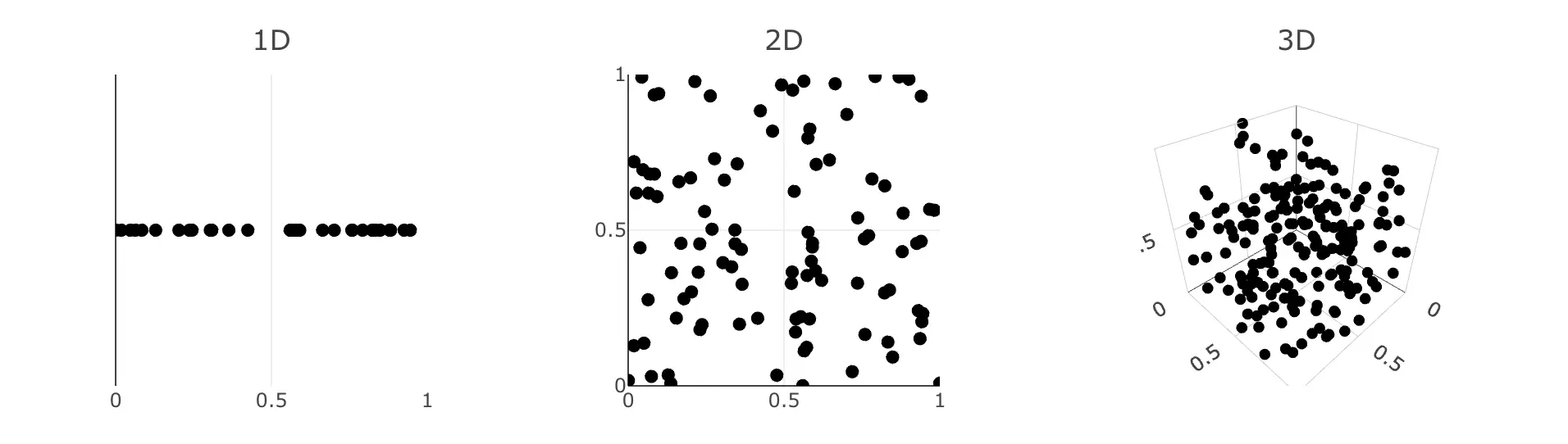
Puseudo-random noise usually don't produce good uniform samples. It often produces clusters and void within the sample space. That means the sample space is not well explored, either wasting samples on similar areas or even complete ignoring some subregions. And this scales to any dimensions.
Stratified Sampling
Instead of recklessly scatter points around, how about subdiving the domain \(\Omega\) into non-overlapping regions \(\Omega_1, \dots, \Omega_n\). Noted that the union of them must cover the whole domain.
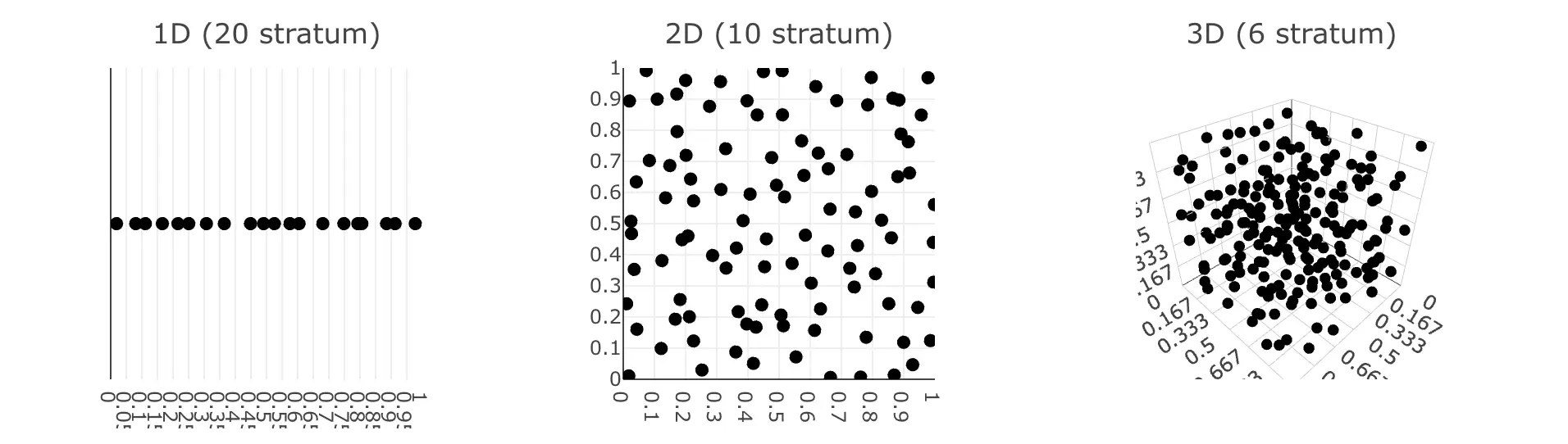
This works pretty well in low-dimensional integration problems. However unfortunately, this suffers the same problem as the quadrature rules where it won't perform well in high frequency signals.
Low-Discrepancy Sequences
If randomness are difficult to control, how about herding the points to position in a deterministic pattern such that they are almost equal distance to each other? In other words, how do we get an equidistribution of samples?
Defining Discrepancy
Imagine a \(s\)-dimentional unit cube \(\mathbb{I}^s = [0, 1)^s\), with a point set \(P = {x_1, x_2, \dots, x_N} \in \mathbb{I}^s\). We define the point set discrepancy1 \(\mathcal{D}(J, P)\) as follows:
You can think of \(\mathcal{D}(J, P)\) as the proportion of points inside a sub-interval \(J\), where \(A(J)\) is the number of points \(x_i \in J\) and \(V(J)\) is the volume of \(J\).
The worst-case discrepancy is called the star-discrepancy and is defined as:
A good sequence should minimize such star-discrepancy \(\mathcal{D^*}(N)\) to be qualified as low-discrepancy. Perhaps it's easier to visualize the terms in a diagram.
\(N=\) \(\mathcal{D}(A, P) =|\)\(\frac{A(A)}{N}-V(A)\)\(|=\) \(\mathcal{D}(B, P) =|\)\(\frac{A(B)}{N}-V(B)\)\(|=\) \(\mathcal{D}(C, P) =|\)\(\frac{A(C)}{N}-V(C)\)\(|=\) \(\mathcal{D^*}(P) =\)
Halton Sequence
One of the well-known low discrepancy sequences is generated using the radical inverse of numbers. They are called radical inverse sequence, and is defined as:
where \(b\) is the base and \(d_k\) is the \(k\)-th digit in the \(b\)-ary expansion of \(n\). To generate a sequence for \(b=2\), first represent the natural numbers in binary, then revert the digits and take its inverse. i.e.
This is also known as the van der Corput sequence2, a specialized one-dimensional radical inverse sequence. The generalized form is called the Halton sequence, that is scalable to higher dimensions. To generate points in \(N\)-dimension, simply pick a different base from the prim number series \({2, 3, 5, 7, 11, \dots}\). Scratchapixel has a more in-depth explanation, feel free to give it a read!
Sobol Sequence
Progressive Multi-Jittered Sample Sequence3
-
Dalal, I., Stefan, D., & Harwayne-Gidansky, J. (2008). Low discrepancy sequences for Monte Carlo simulations on reconfigurable platforms. In 2008 International Conference on Application-Specific Systems, Architectures and Processors (pp. 108–113). ↩
-
van der Corput, J.G. (1935), "Verteilungsfunktionen (Erste Mitteilung)" (PDF), Proceedings of the Koninklijke Akademie van Wetenschappen te Amsterdam (in German), 38: 813–821, Zbl 0012.34705 ↩
-
Christensen, P., Kensler, A., & Kilpatrick, C. (2018). Progressive Multi-Jittered Sample Sequences. Computer Graphics Forum. ↩